


发布时间:2024-06-04 17:46:25 作者:佚名 点击量:
可以是一本书,也可以是几本循序渐进的书,中文英文皆可,如果Springer能找到或者有别的电子书就更好啦。希望包括以下内容的理论和应用:
单目标、多目标、线性、非线性问题的优化,遗传算法、粒子群算法、模拟退火算法等优化算法,寻优方式(寻优方向和收敛准则)。
这么全方面的吗?
那我大概只能强推算法禁书目……啊呸算法导论了
实在是高数课上打发时间编译同时压泡面的不二良品。
顺便大概还可以防切防隔防击打
如果把它一家都带上也是好的
(我们当中出了一个奸细~)
开门见山,先说我觉得挺重要的几本书,然后会结合自己的学习体会说明原因。
一、书籍简介
对于目前的我来说,这四本书分别对应科研能力的3个方面:实际问题抽象及建模、算法理论和数据结构、算法实践(动手能力)。《数学建模》中包括常见基本的优化算法(其实优化只是其中一小部分),
搞自动驾驶感知方面的研究近两年,随着研究深入,逐渐感觉到想要真正创新性解决一些实际问题甚至难题,就要能够深入透彻地理解问题;然后基于一定假设对工程中的实际问题进行抽象,建模成为数学问题;再是通过一定理论层面的算法设计来解决问题;最后则是需要将理论层面的算法通过代码来落地实现。在有挑战的科研任务中,这4个步骤都会有很大影响。
所以,我目前先推荐以上这几本。当然,结合我目前的理解和研究阶段而言基本够用,如果以后有新的认知会来更新,也欢迎大佬补充。
以下则是书籍链接,经典的纸质书值得经常翻,重要的是多思考。
最后一个 Leetcode在github上有大佬写的书。以下是链接
GitHub - azl397985856/leetcode: LeetCode Solutions: A Record of My Problem Solving Journey.( leetcode题解,记录自己的leetcode解题之路。)
这一本,刚发现的,个人认为很实用,对没有基础的同学也友好
Talk about methods that only use first-order information (i.e., the gradient).
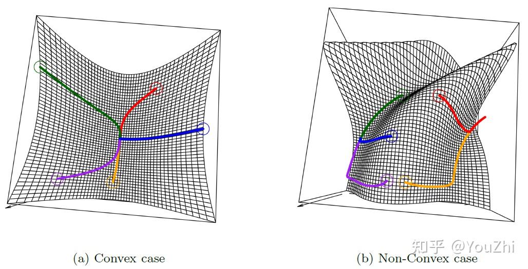
Considering the unconstrained, smooth convex optimization
We assume a few thing about the function :
Under this assumption, we denote the optimal criterion value by
with the solution at .
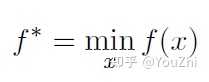
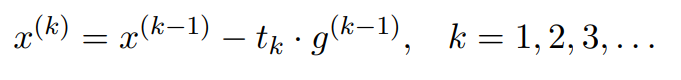
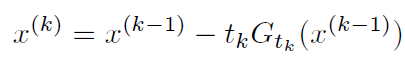
The Gradient Descent algorithm is then de ned as follows:
Above, after choosing some initial point , we move it in the direction of the negative gradient (this points us in a direction where the function is decreasing) by some positive amount
, calling this
. And the same process is repeated.
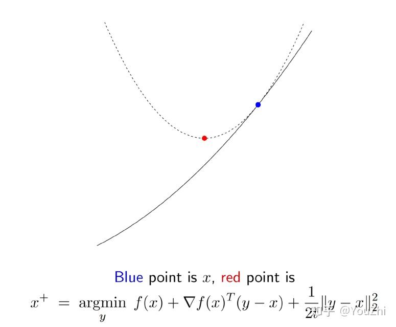
The second-order Taylor expansion of f gives us
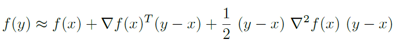
Consider the Quadratic approximation of , replacing
by
(replacing the curvature given by the Hessian with a much simpler notion of curvature - something spherical), we have
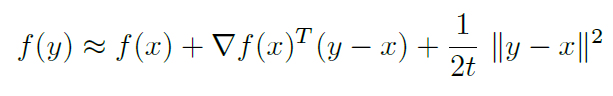
Minimizing this w.r.t. , we get
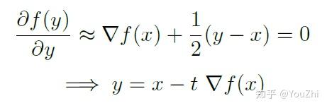
This gives us the gradient descent update rule. In other words, gradients descent actually chooses the next point to minimize this overall .
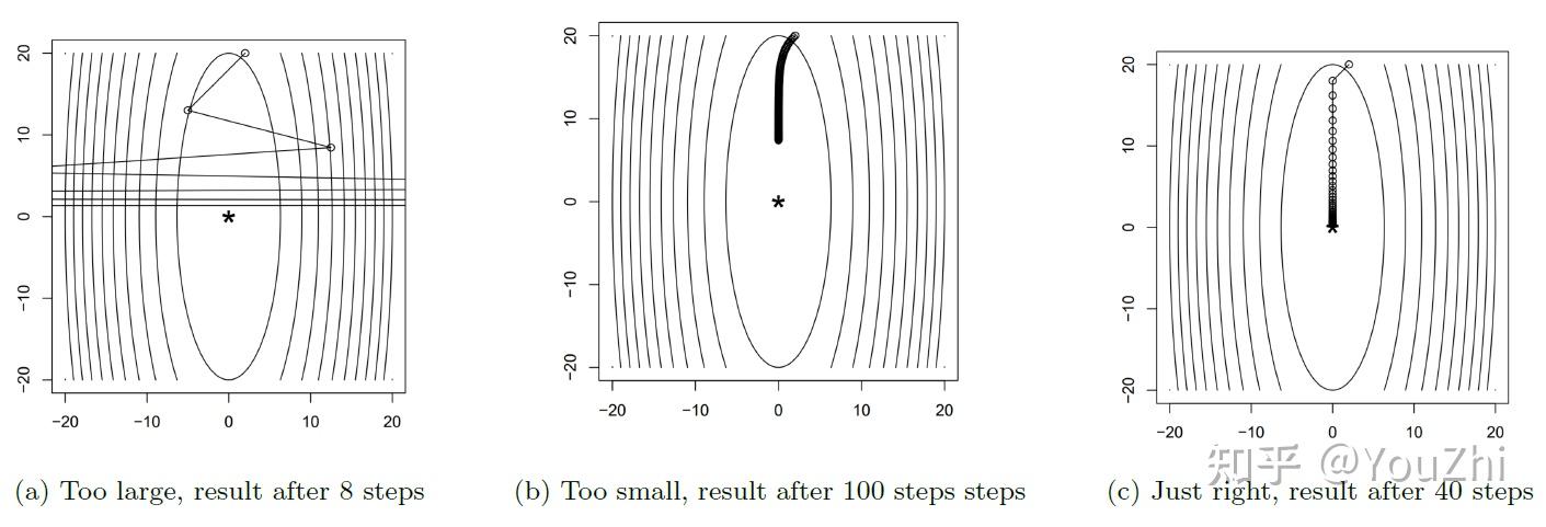
Fixed step size
The simplest strategy is to take the step sizes to be fixed. So we choose ; for all
There are some problems with doing this:
Functions tend to converge nicely only when t is "just right", as we can see below.
Backtracking Line Search
Using adaptive step sizes - not just something fixed, but instead trying to guess the right step size at every iteration via some heuristic.
The most popular such heuristic is called Backtracking Line Search. This works as follows:
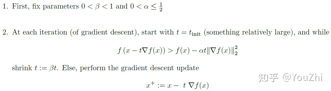
The update criterion above denotes that, if the progress we make by going from to
is bigger than the progress we had
, then we make
smaller
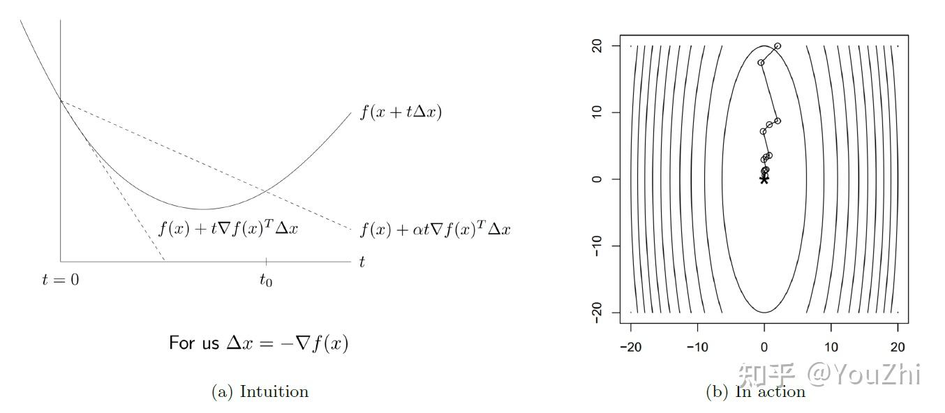
.
So by shrinking , we move from right to left on the graph, as long as the line is beneath the function, and then stop when it exceeds it.
Exact Line Search
We could also choose a step to do the best we can along the direction of the negative gradient, called Exact Line Search:
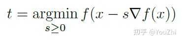
is fi xed above (its the point we're currently at during gradient descent), and we find the value of
that allows us to do the absolute best we can along that line segment.
Trying to make this as small as possible over all s is a 1-dimensional optimization problem. In principle, we might think its a good idea to optimize this.
But this is usually not possible to do directly; and approximations to the same are not as efficient as general backtracking. So is not worth the effort (except for fairly simple problems maybe).
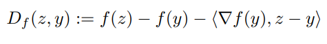
is a subgradient of a convex function
at
if
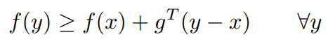
经过点 的linear approximation
always underestimates
.
Some properties of subgradients:
? Always exists in the relative interior of the dom( ).
? If is indeed differentiable at
, then
uniquely.
? This definition is universal - can hold for non-convex functions too. However, it could be possible that doesn’t exist.
The subdifferential of a convex function at
is the collection of all subgradients of
at
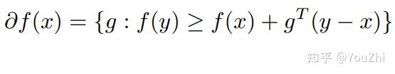
Some properties of the subdifferential:
? For convex ,
. However, for concave
,
.
? is closed and convex for any
.
? Since the subgradient is unique at points of differentiability, when
is differentiable at
.
? is singleton, then
is differentiable at
and
is that only element of
.
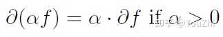
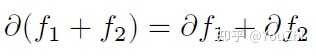
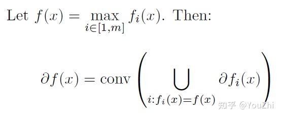
Some basic rules for convex functions and their subgradients / subdifferentials:

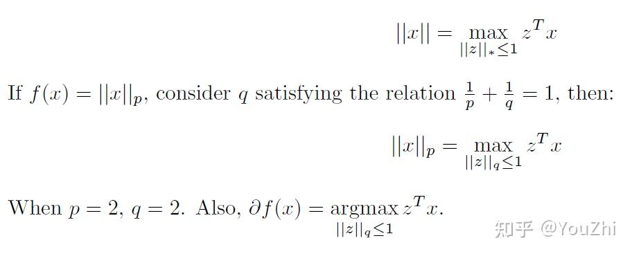
To each norm , there is a dual norm
such that:
Now consider convex, having
, but not necessarily differentiable.
Like gradient descent, but replacing gradients with subgradients.:
where , any subgradient of
at
.
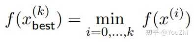
Subgradient method is not necessarily a descent method, thus we keep track of best iterate among
so far, i.e.,
Step size choices

Key difference to gradient descent: step sizes are pre-specified, not adaptively computed.
Subgradient method has convergence rate , slower than
rate of gradient descent.
Solving the following convex minimization problem
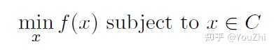
Using projected subgradient descent.
It has the same update as the subgradient method, except we project onto instead of calculating the subgradient at each step
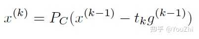
If this projection can be done, the projected subgradient method achieves the same convergence guarantees as subgradient descent.
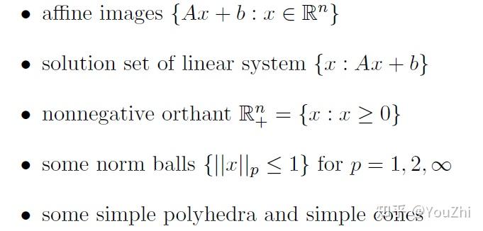
However, some projections are easy (e,g, for projecting x onto the norm, just divide
by its
norm). Some other easy projections are:
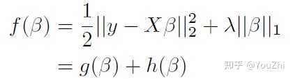
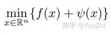
Minimizing composite functions of the form
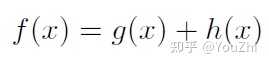
where is convex and differentiable, and
is simple and convex but nonsmooth. This relaxes the class of functions we can minimize compared to gradient descent, but for many problems we can still achieve the
rate of convergence from gradient descent.
Since h is not differentiable, we cannot directly take the gradient descent update. Instead, we can try another method motivated by the same principles as gradient descent. Recall that the gradient descent method is motivated by minimizing a quadratic approximation to around
, replaying the Hessian with
.
Instead of trying to minimize the quadratic around all of , which we can't do because
is not differentiable, we can minimize just the quadratic approximation to
and leave
alone. Make the update:
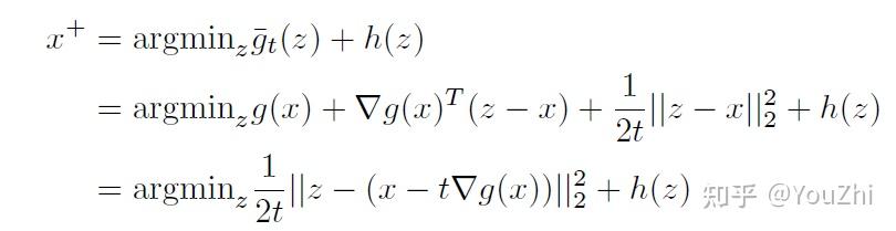
The fi rst term forces us to stay close to the gradient update for
and the second terms forces us to make
small. This is the principle behind proximal mapping.
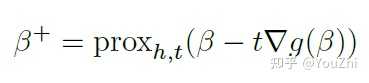
Proximal mapping is given by
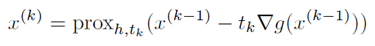
proximal gradient descent:
1.choose an initial
2. iteratively update (Proximal gradient (PG))
rewrite in the same form as a gradient step by defi ning
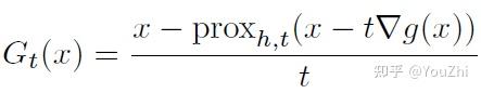
rewriting the update as:
The advantage of the proximal mapping is that has a closed-form solution for many important functions
, which may not be differentiable but are simple. Making the proximal mapping only depends on
, and because
is smooth we can compute its gradients even though it may be very complicated. The computational cost of making the mapping, however, depends on the function and can be either expensive or cheap.
Example:
lasso criterion
the proximal mapping for is
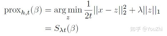
where is the soft thresholding operator:
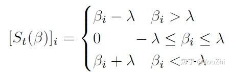
The proximal update is

Using the fact that and the de nition of
.
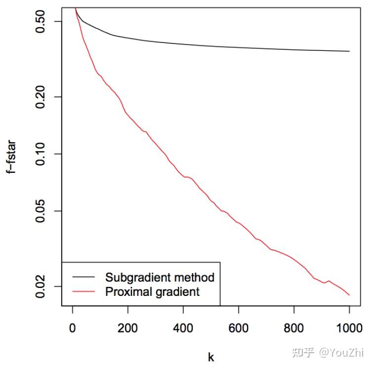
Semonstrating the faster convergence speed of the proximal gradient method over the subgradient method in the following graph:
Backtracking works the same as it does for gradient descent, but because we require the derivative we use backtracking only on , not
. Choose a parameter
. At each iteration start at
and while

shrink the step size . Otherwise perform the proximal gradient update.
| Stochastic gradient descent |
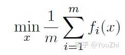
Consider the following problem of minimizing an average of functions:
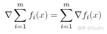
The gradient of the above objective function will be
If we apply gradient descent algorithm, we would be repeating the following steps:
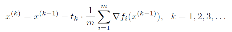
However, gradient descent will be very costly if we have in the order of, say, 1 millions.
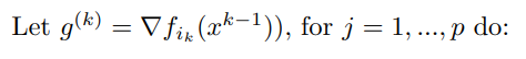
Stochastic gradient descent or SGD (or incremental gradient descent):
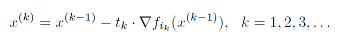
where is some chosen index at iteration
.
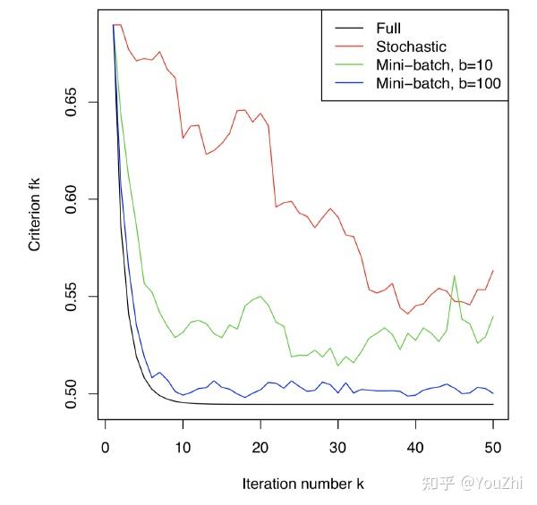
Choosing Index
there are two ways:


Step Sizes
It is standard to use diminishing step sizes in SGD (e.g., ).
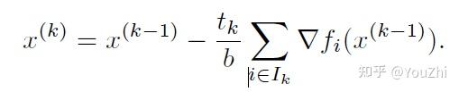
During the -th update, we choose a random subset
, where
, and use the following update rule:
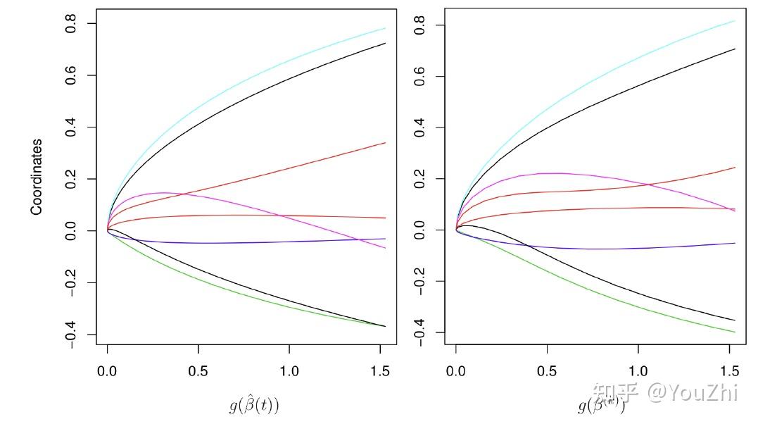
It turns out that solve a regularized logistic regression:
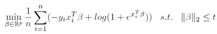
is similar to running gradient descent on the unregularized problem:

and stop early.
By "early", it means to stop really early instead of stopping when we are bouncing around
the minima.

With early stopping, it is both more convenient and much more effcient than using explicit regularization.
Because in this way, it does not require running with different parameter , just running gradient descent.
And it turns out when we plot gradient descent iterates, it resembles the solution path of the regularized problem for varying
!
Generalizing the Euclidean proximal map to the Bregman proximal map.
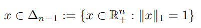
Consider the problem:
where is differentiable and convex, and
is closed and convex with
. Note that
tends to be a regularization term.
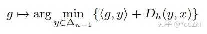
Bregman proximal map
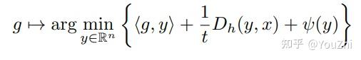
The idea here is to replace with
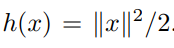
. The Euclidean proximal map previously corresponds to the squared Euclidean norm reference function
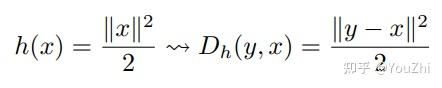
Suppose is a reference function. The Bregman proximal gradient (BPG) method does:
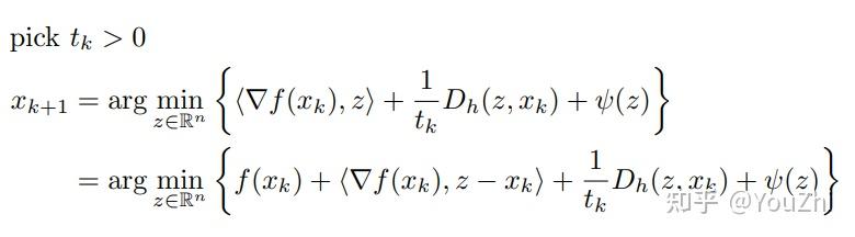
Convergence. Bregman proximal gradient has convergence when
is smooth relative to
, i.e., when
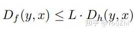
for all .
By generalizing the reference function beyond the Euclidean squared norm, bregman proximal methods attain additional freedom which may aid the computation of the proximal mapping.
For example,
the map
is much simpler for
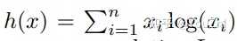
than for
We will generalize the L-smoothness assumption for convergence to relative L-smoothness.
| Modern stochastic methods |
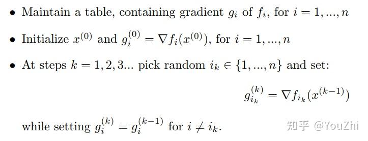
Stochastic average gradient
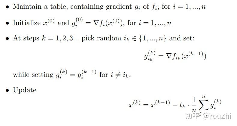
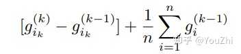
For the update step, at each iteration, it only requires an O(1) addition for the aggregate gradient from the previous step to be modified to become the aggregate gradient for the current step:
The above update can be seen as a moving average over a sliding window which is a constant time calculation.
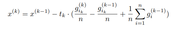
SAGA
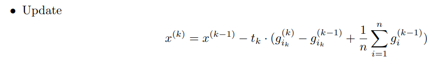
Notice that the only difference between SAG and SAGA is the heavier weight on the updated gradient at step . We have:
instead of
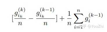
SAGA matches convergence rates of SAG.
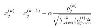
The advantage of the above update rule is that, we do not need to tune our learning rate anymore as is now a fixed hyperparameter.
It is noted that in sparse problems, AdaGrad performs much better than standard SGD. Several extensions of AdaGrad exists, viz., Adam, RMSProp etc.
[1]
https://www.stat.cmu.edu/~ryantibs/convexopt/微电网优化模型介绍:
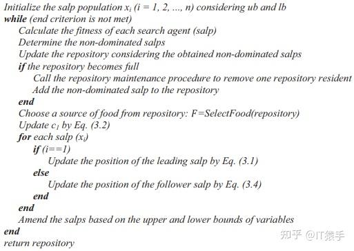
多目标鳟海鞘算法(Multi-objective Salp Swarm Algorithm,MSSA)由Seyedali Mirjalili等人于2017年提出。
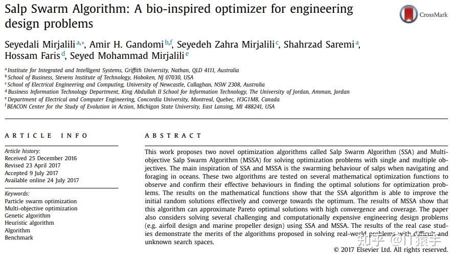
参考文献:S. Mirjalili, A.H. Gandomi, S.Z. Mirjalili, S. Saremi, H. Faris, S.M. Mirjalili,Salp Swarm Algorithm: A bio-inspired optimizer for engineering design problems ,Advances in Engineering Software. DOI: http://dx.doi.org/10.1016/j.advengsoft.2017.07.002
close all;
clear ;
clc;
global P_load; %电负荷
global WT;%风电
global PV;%光伏
%%
TestProblem=1;
MultiObj=GetFunInfo(TestProblem);
MultiObjFnc=MultiObj.name;%问题名
% Parameters
params.Np=200; % 种群大小(可以修改)
params.Nr=params.Np ; % (外部存档的大小)
params.maxgen=200; % 最大迭代次数(可以修改)
[Xbest,Fbest]=MSSA(params,MultiObj);
% Xbest是算法所求得到的POX
% Fbest是算法所求得到的POF
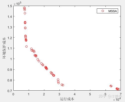
%% 画结果图
figure(1)
plot(Fbest(:,1),Fbest(:,2),'ro');
legend('MSSA');
xlabel('运行成本')
ylabel('环境保护成本')
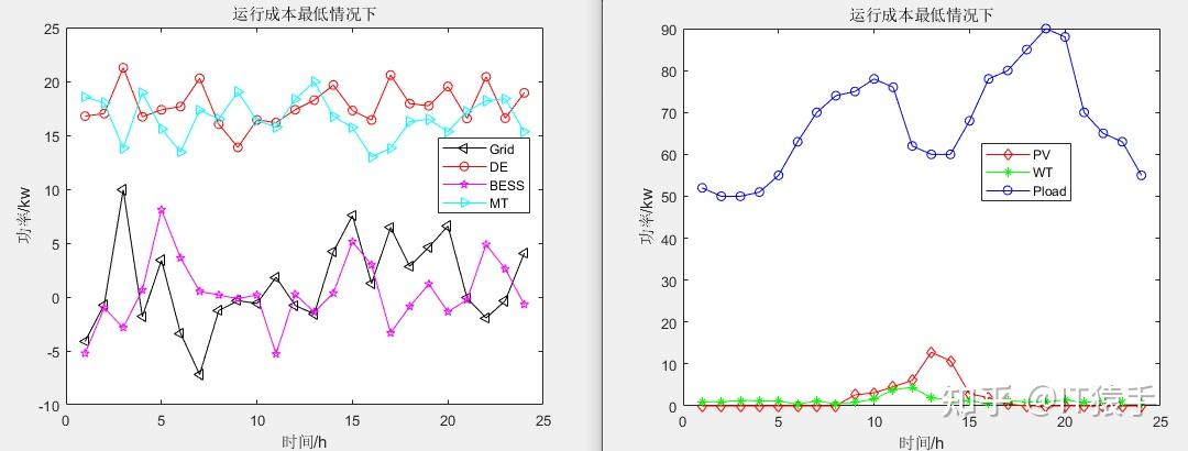
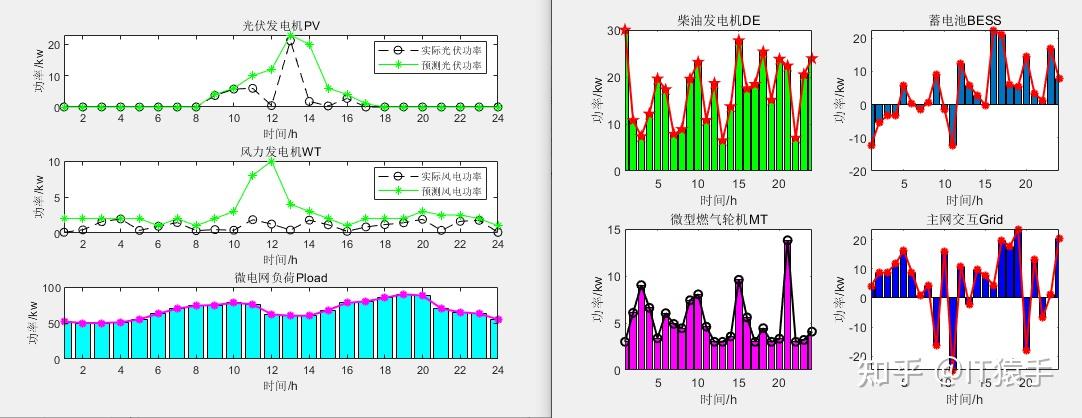
a)运行成本最低情况下:
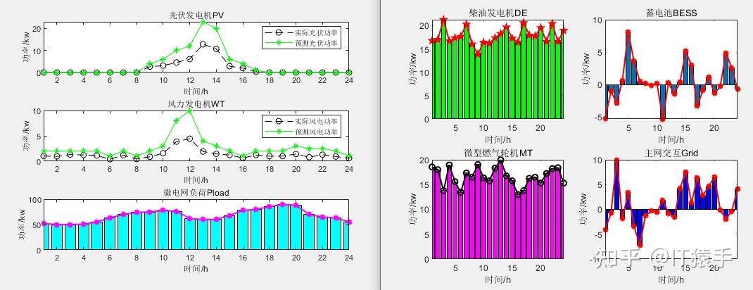
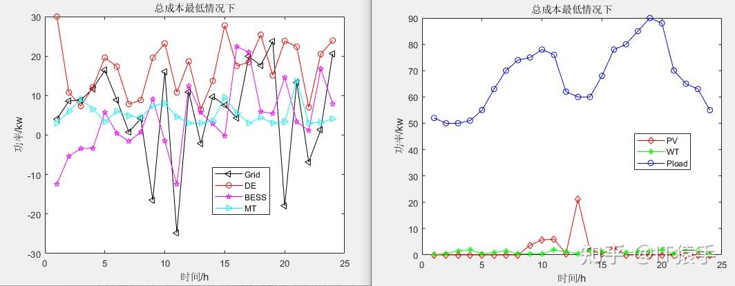
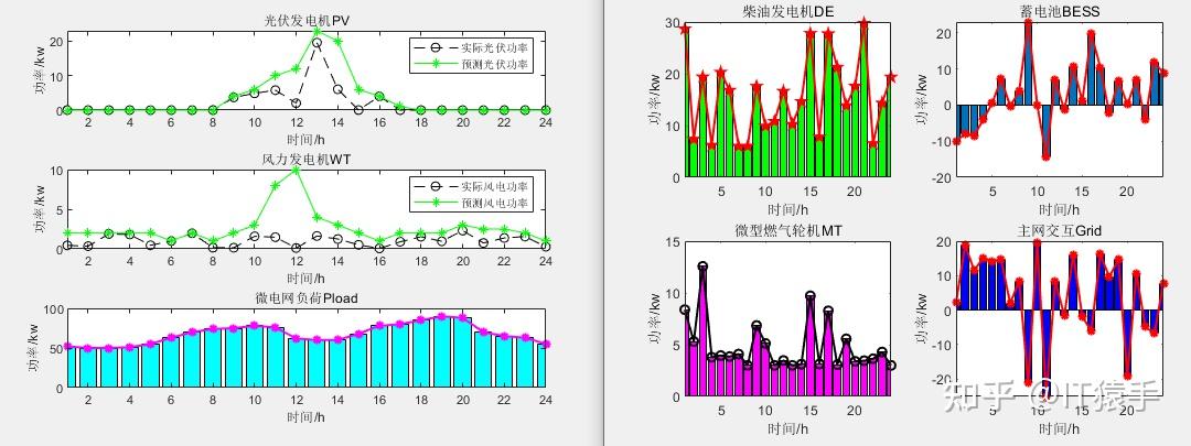
b)总成本最低情况下:
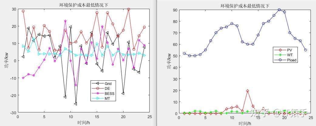
c)环境保护成本最低情况下:
基于瞪羚优化算法(Gazelle Optimization Algorithm,GOA)求解微电网优化MATLAB - 知乎 (zhihu.com)
单目标应用:基于沙丁鱼优化算法(SOA)的微电网优化调度MATLAB - 知乎 (zhihu.com)
单目标应用:基于螳螂搜索算法(Mantis Search Algorithm,MSA)的微电网优化调度MATLAB - 知乎 (zhihu.com)
单目标应用:基于狐猴优化算法(Lemurs Optimizer,LO)的微电网优化调度MATLAB - 知乎 (zhihu.com)
多目标应用:基于多目标向日葵优化算法(MOSFO)的微电网多目标优化调度MATLAB - 知乎 (zhihu.com)
单目标应用:霸王龙优化算法(Tyrannosaurus optimization,TROA)求解微电网优化MATLAB - 知乎 (zhihu.com)
单目标应用:基于蜘蛛蜂优化算法(Spider wasp optimizer,SWO)的微电网优化调度MATLAB - 知乎 (zhihu.com)
单目标应用:基于淘金优化算法(Gold rush optimizer,GRO)的微电网优化调度MATLAB - 知乎 (zhihu.com)
单目标应用:基于成长优化算法(Growth Optimizer,GO)的微电网优化调度MATLAB - 知乎 (zhihu.com)
基于麻雀搜索算法SSA的微电网优化调度MATLAB - 知乎 (zhihu.com)
多目标应用:基于多目标哈里斯鹰优化算法(MOHHO)的微电网多目标优化调度研究MATLAB - 知乎 (zhihu.com)
多目标应用:基于多目标人工蜂鸟算法(MOAHA)的微电网多目标优化调度研究MATLAB - 知乎 (zhihu.com)
猎豹优化算法(The Cheetah Optimizer,CO)求解微电网优化MATLAB - 知乎 (zhihu.com)
遗传算法(Genetic Algorithm,GA)求解微电网优化MATLAB - 知乎 (zhihu.com)
蚁群算法(Ant Colony Optimization,ACO)求解微电网优化MATLAB - 知乎 (zhihu.com)
墨西哥蝾螈优化算法(Mexican Axolotl Optimization,MAO)求解微电网优化MATLAB - 知乎 (zhihu.com)
联系我们
contact us
地址:广东省广州市天河区88号

电话:400-123-4567

点击图标在线留言,我们会及时回复